
“You don’t need the source to understand the story. Every visual is a clue. Every field is evidence.”
The Reverse Engineer’s Mindset
The developer is gone. The .pbix is locked. The deadline is tomorrow. This is how you reverse engineer your way out.
When someone hands you a Power BI report with no source files, no developer, and no access to the .pbix, you have two options: rebuild from scratch and guess — or reverse engineer what is already there.
This guide covers the second approach. Starting from nothing but report screenshots, you will work through every visual, extract every field name, classify each one, and construct a normalized, production-ready star schema that validates against the report itself. Seven steps. One clean data model.
What You Need Before You Start
Before jumping into the framework, make sure you have these four things ready:
- Report Screenshots: Full-page captures of every tab, including filter panes and tooltips where visible. The more complete your screenshots, the more accurate your schema will be.
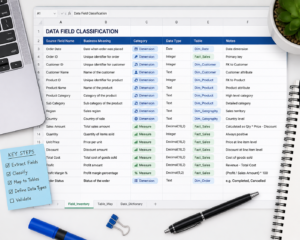
- Field Inventory Sheet: A spreadsheet to log fields, types, visual source, and classification status at each step. This becomes your single source of truth throughout the process.
- DAX Knowledge: Basic familiarity with DAX patterns to separate base measures from calculated or time-intelligence measures. You don’t need to be an expert you just need to recognize the difference.
- Schema Design Tool: dbdiagram.io, Lucidchart, or Power BI Desktop to sketch and validate the star or snowflake schema as you build it.
The 7-Step Reverse Engineering Framework
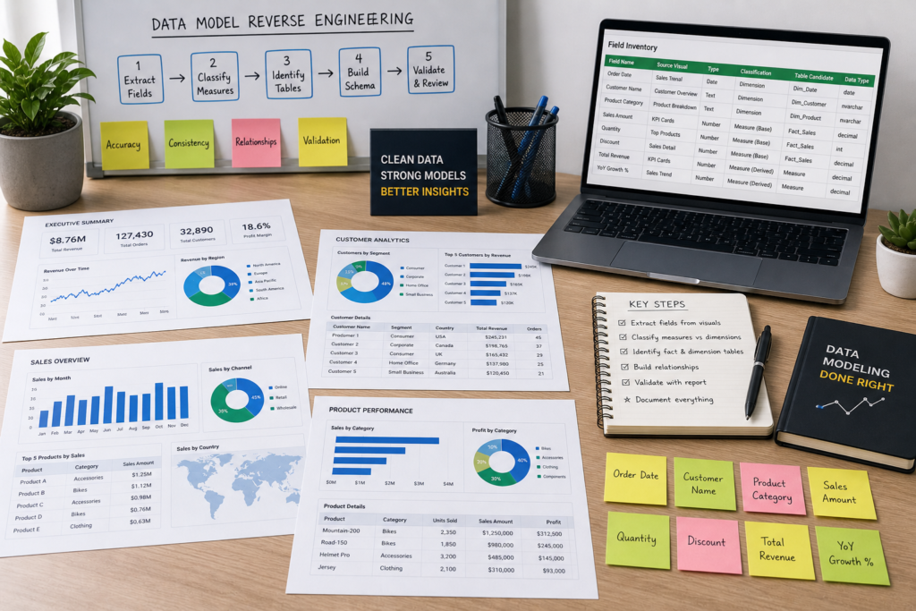
Step 1: Find Fields Used in Each Visual
Go through every chart, table, card, and slicer in the screenshots. Record each field name exactly as it appears: axis labels, legend entries, tooltip fields, and filter pane items. Do not paraphrase or clean up names yet capture exactly what is shown. This raw list is your starting material for everything that follows.
Step 2: Normalize the Field List
Standardize naming conventions. Remove display formatting, title casing, and abbreviations. Map each field to a clean, consistent name so duplicates across visuals become visible. For example, “Sales Amt”, “SalesAmount”, and “Total Sales” might all refer to the same column normalization reveals that.
Step 3: Deduplicate Across Visuals
Fields appear in multiple charts. Collapse the full list into one unique set: one row per field. This prevents modeling the same attribute twice under different visual labels. By the end of this step you should have a clean, flat list of every unique field in the report – no repeats.
Step 4: Filter Measures vs. Dimensions
Split your field list into two buckets. Measures are aggregated numerics Sum of Sales, Count of Orders, Average Revenue. Dimensions are categorical attributes used to slice and filter Region, Product Name, Date, Customer Segment. If a field is used on an axis or as a slicer, it is almost always a dimension. If it appears as a value or KPI card, it is almost always a measure.
Step 5: Separate Base from Derived Measures
Base measures are direct column aggregations SUM(Sales[Amount]), COUNT(Orders[OrderID]). Derived measures are calculated on top of base values using DAX Revenue YTD, Win Rate, Profit Margin %. Identifying this layer lets you reconstruct DAX logic in the correct order. Always build base measures first, then layer derived measures on top.
Step 6: Separate Fact Tables from Dimension Tables
Group dimensions by entity: time, product, customer, geography. These become your dimension tables. All transactional numeric data and foreign keys go into fact tables. A typical result looks like this:
- FACT_SALES: OrderID, Amount, FK to all dimensions
- DIM_DATE: Year, Quarter, Month
- DIM_PRODUCT: Name, Category
- DIM_CUSTOMER: Segment, Region
- DIM_REGION: Country, City
- DIM_SALESREP: Name, Team
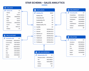
Step 7: Build a Star or Snowflake Schema
Wire fact and dimension tables together. Define primary keys in dimension tables and foreign keys in the fact table. Choose a star schema for flat dimensions one level of lookup tables. Choose a snowflake schema for hierarchical ones where dimensions reference other dimensions. Validate every field against the report visuals. If a visual cannot be reproduced from your schema, you have either a missing table or a misclassified measure.
What You Can Achieve
By following this framework you can:
- Recover data models from legacy reports with no documentation
- Create a clean migration path to a new BI platform
- Produce a reproducible schema from any set of screenshots
- Maintain clear separation of base vs. derived DAX logic
- Reduce rework when rebuilding reports from scratch
- Deliver auditable measure logic with no guesswork
- Produce a production-ready star schema in a single session
- Fully document undocumented dashboards before migration
Who This Framework Is Built For
For the Data Engineer: Structured field extraction process with no ambiguity. Clear rules for separating fact and dimension tables. Schema output that maps directly into your data warehouse. Reproducible results across any Power BI report.
For the BI Developer: Step-by-step measure classification for DAX reconstruction. Logical separation of base measures from calculated ones. Schema you can load directly into Power BI Desktop. A validation layer to confirm every visual is reproducible.
For the Business Analyst: Understand which fields drive each KPI in the report. Document legacy dashboards before migration. Communicate field-level requirements to the dev team. Catch discrepancies between what reports show and what the data actually says.

The Complete 7-Step Flow
Audit Visuals → Extract Fields → Normalize and Dedup → Classify Measures → Split Fact and Dims → Build Schema → Validate Output
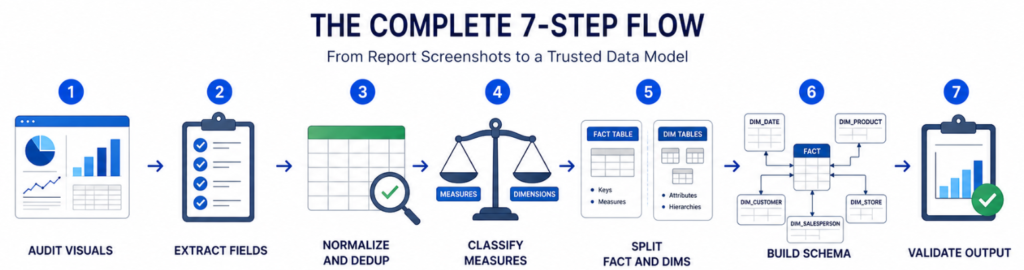
Each step builds directly on the last moving from raw field names visible in report visuals all the way to a validated, normalized schema ready for production.
Start Your Reverse Engineering Project Today
The next time someone hands you a Power BI report with no source, no developer, and no documentation you have a framework. Work through each visual, one field at a time. The data model is already there. You just need to uncover it.